MacroGranometer™ is a computerized sedimentation analyzer of water-insoluble, sand-sized material, using
gravity sedimentation from a single level (stratified
sedimentation) in water. Employing the most sophisticated solutions
makes it the unique tool for sand sedimentology,
which provides high quality and meaningful results, with added operational and maintenance ease, and
a variety of outputs.
MacroGranometer™ measures the
sedimentation velocity distribution,
and its data processing program, SedVar™, converts it into a distribution of
other sedimentation
variables, such as shape-specified grain size. For the conversion, the equation for drag coefficient as a function
of Reynolds' number and grain shape developed by J.
Brezina (1979b) is utilized.
Distributions of the
following sedimentation variables are
available:
- sedimentation velocity, in three versions:
- laboratory
- standard
- local
- shape-specified grain size
- grain shape
- grain density
- Reynolds' number
The grain parameters density and
shape
can each be quantified as a distribution. This is possible
from samples of nearly equal grain size such as narrow sieve
fractions.
Our processing software SedVar™ also computes distributions of the grain
sedimentational Reynolds' number; these distributions, similarly
to those of PSI sedimentation velocity, feature a less negative skewness than
the pertinent PHI grain size distributions. In fact, the skewness of the grain
sedimentational Reynolds' number distributions has a medium value between the
most negatively skewed PHI, and least negatively skewed PSI distributions).
Not only that our Reynolds' number distributions use the shape-specified grain
size but can be computed for samples of nearly equal grain size (narrow sieve
fractions with varying grain density), and for nearly equal grain density.
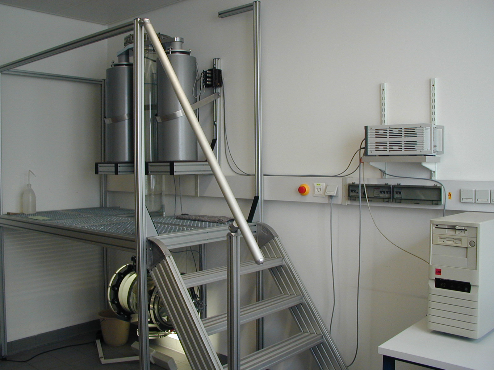
The MacroGranometer™ system is shown on the
schematic view below:
|
|
3a
GRM™, Measuring & Operational Software
example of the GRM™ analysis window
(User's 486 66
MHz DX2 PC or higher, with 1 LPT and 1 COM interfaces)
2
Control & Measuring Electronic Box
CFM automatic digital amplifier, control
& sensor PCBs,
power supply, cable distributor
3b
SedVar™, Processing Software
|
|
The schematic view of the
MacroGranometer™
the sedimentation length L is usually 180 cm |
|
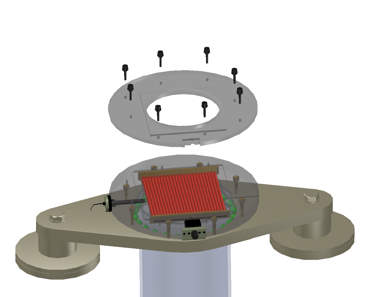
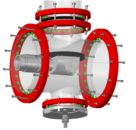
3-D view
of the
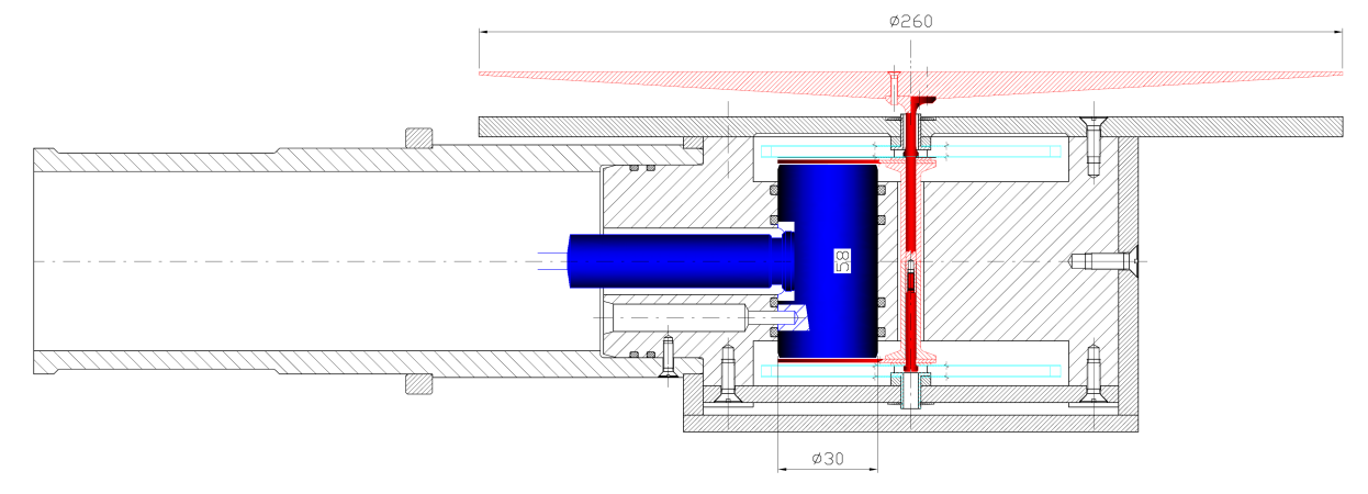
Upper Part of the Sedimentation Tube: Venetian Blind (sample introduction)
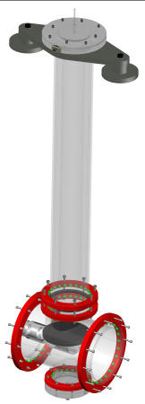
3-D view of the MacroGranometer's™
Sedimentation Tube
(larger view: klick) |
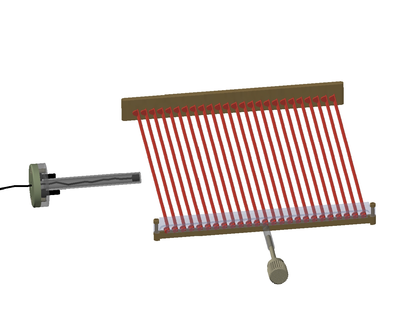
Open
lamellae of the Venetian Blind
(without rotational magnet etc.)

Underwater Balance Body
(larger view: klick) |
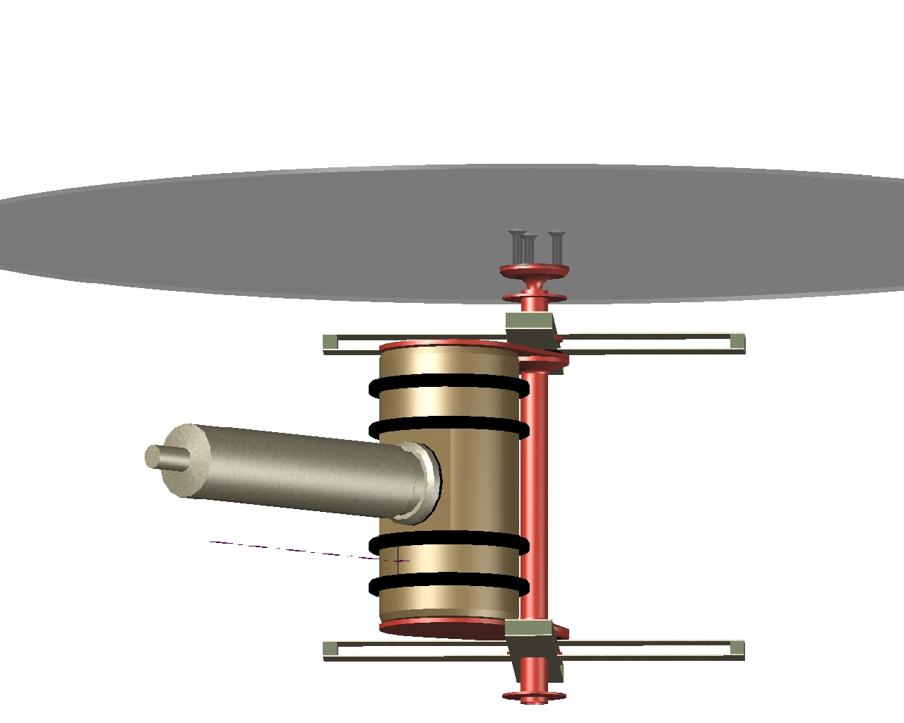
3D-View of the Underwater Balance Body
3-D view
of the
Lower Part of the Sedimentation Tube with the
Underwater Balance
(larger view: klick) |
|
Our measuring software
GRM™ runs on the user's 486 DX2 66 MHz PC or higher, under MS DOS 6.2 or higher. It controls the system's operation and stores the
measured data as ASCII files.
Our processing software
SedVar™ runs on the user's MS Windows
98 PC or higher. It processes the measured PSI local sedimentation velocity
distributions.
SedVar™ consists of three parts:
- SedVar™, distribution conversion,
- SedGraph™,
graphical output
generator,
- Sed 3D Graph™,
3D plot of a multiple distribution graph.
|
|
MEASURING RANGE: |
0.016 - 4 mm |
|
quartz
density materials: |
0.044 - 4 mm |
|
heavier materials: |
may be finer, such as 0.016
- 1 mm; |
|
SAMPLE SIZE: |
smallest, statistically representative
samples of
15,000 - 20,000 grains (0.1 - 5 gram); |
|
settling rate resolution: |
0.02 PSI |
|
weight resolution: |
0.01 % |
RESULTS: semi graphic and full graphic print-outs showing distributions
of the six sedimentation variables listed above, such as laboratory, standard and local
PSI sedimentation velocities, PHI grain
size, density, shape factor and Reynolds' number including either variable size, density
or shape factor. The standard sedimentation velocity and Reynolds' number are available also for
sieve fractions (constant size) and heavy liquid fractions
(constant size and density);
each variable is resolved into 401 logarithmically equidistant intervals.
Mean, spread,
asymmetry & peakedness are calculated as
moment and percentile distribution
characteristics of each variable. Other characteristics may be included as
you wish.
The program
Sed 3D Graph™ (part of the SedVar™ program) permits a graphical display of a
group of
distributions, either according to the samples' geographic
horizontal or vertical location, or according to another desired variable. For
example, a group of PSI-settling velocity (or grain density) distributions, each
from a constant grain size fraction, can be plotted according to their PHI-grain
size.
The optional program
SHAPE™ provides the possibility of
separating as many as five mixed distribution components, each normally
distributed. This program can match a sieve analysis to the sedimentation analysis of the same sample, and compute Shape Factor values
to each
0.02-PSI sedimentation velocity. Our SedVar™ program can use this set of the
variable
SF values to adjust the sedimentation grain
size distributions of similar samples (the results of the MacroGranometer™) to the
sieving; in
other words, it can simulate the sieving errors.

Examples
of our clients
who use the instrument
-
Department of Geological Sciences,
University of Trieste, Italy (click);
-
Department of Geology, University
of Vienna, Austria (click).
Example of a PSI distribution decomposed into Gaussian components
SAMPLE:
FileName:
sed122.dat
A sand
fraction, consisting of nearly monosize grains, made by precision sieves with
circular holes:
|
Material:
|
black sand
|
sample 13
|
at a 90° intersection of beaches
|
|
Locality:
|
near Casusay
|
Venezuela Bay
|
about 110 km NNW of Maracaibo
|
|
Sampling Date:
|
1972-5-15
|
low tide
|
tide amplitude: about 75 cm
|
|
Analysis date, time:
|
1981-2-1, 16:55h
|
Tmean
= 24.76°C
|
|
Preparation:
|
precision wet vibration sieving
|
circular holes ± 0,002 mm
|
|
MonoSize:
|
1.770 ±0.0639 PHI
|
= 0.297 ±0.013 mm
|
|
Average of 8 sample
split analyses:
|
Total Mass:
Mean Sample
Split Mass:
|
0.6916 gram
0.08645 gram
|
SF = 0.63 (calculated Corey‘s Shape Factor)
Glab = 980.962 gal (cm/sec2)
|
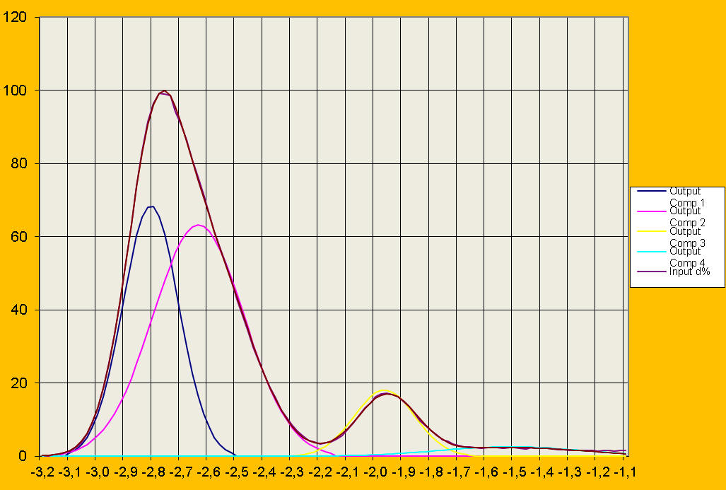
PSI Distribution
of
MonoSize
(1.77PHI=0.297mm)
Polymineral
Fraction
Decomposed into
4 Gaussian Components
Our Sand Sedimentation Analyzer™
(MacroGranometer™)
measured at 0.02 PSI intervals (X-axis).
No data manipulation such as “smoothing“ has been used.
The smoothness
of the 1st derivative,“Input d%“, shows the
analysis quality.
Our Program SHAPE™
identified
4 Gaussian Components (Comp
1,
Comp 2,
Comp 3
and Comp 4).
Our
Program SHAPE™
(based on the method by Isobel CLARK,
1977)
decomposed
the analyzed
PSI
distribution into
4
Gaussian
components
with the following 11
parameters
-
4 means, 4 standard deviations, 3 percentages
(the 4th one is the rest up to 100%):
|
#
|
PSI-mean
|
St. Dev.
|
%
|
Density
|
Minerals
(calculated & confirmed)
|
|
1
|
-2.8095
|
.1007
|
34.56
|
4.76
|
ilmenite
|
|
2
|
-2.6376
|
.1645
|
52.15
|
4.16
|
garnets
|
|
3
|
-1.9685
|
.1090
|
9.90
|
2.65
|
quartz,
feldspars, calcite
|
|
4
|
-1.5137
|
.2601
|
3.39
|
2.08
|
porous
calcite (fossils)
|
|
Goodness of fit
|
Chi-Square:
|
χ2 <0.01
|
Our Program
NGRM™
calculated density from the constant PHI size and each PSI-mean value.
The density
values of each component match the minerals identified microscopically and by
X-ray diffraction analysis.
Our Program SedVar™ converted the variable PSI into
a log
density distribution (not shown here).
The ultimately
lowest Chi-square value, χ2 <0.01,
reveals the
decomposition quality.
Client's preparation
for our installation of the
instrument
The client should build and fix
two steel Bases to carry both the Air Shock
Absorbers, and an operation
platform before our installation. Also, a container with about
100 liter distilled water should be available a few days before our installation
(the container should be positioned above the top of the sedimentation column in
order its water will be warmer, and without dissolved air).
J. Brezina collected and processed the data of the Experiment from 17
participants, however, he did not complete the final processing before the
publication deadline of the book by J. P. M. Syvitski
(click on the author's review of the Syvitski's book
in Basin
Research 4/1992).
Below are shown the calibration results of one of the
MacroGranometer™ users, the participant No. 14 (in the Syvitski's book quoted
under instrument code ST3), in comparison with a precision 0.25-PHI
sieving, made by participant No. 7.
The calibration samples consisted of glass spheres with exactly determined density of each of the five
mixture components; three sand samples were mixtures of up to three components. J. Brezina produced
each mixture component on 65-millimeter screens featuring galvanically deposited
meshes with circular holes, with the aid of random vibration of the glass
spheres in alcohol suspension on each screen. The minimum material on each
screen enabled that only one-layer of spheres has been screened until constant
amount of retained spheres (zero throuput), which resulted into ample sieving time.
The component portions have been
obtained on a high precision rotational sample splitter using the slowest
possible samples' flow. The high statistical representativity of each split was
confirmed by the negligible variation of the weight of each component split.
Still, each sample had a specific percentage of the three components, and, this
way, has been produced exclusively
for each participant.
The percentages of each three sieve fractions of the
Sand 1 are shown in the Table below, column headed by "14" for the
Participant 14 (Syvitski's code "ST3"), who analyzed the sub-sample [split]
4, = "14S1S4") by the MacroGranometer. This sub-sample had a mean density
2.487125 g/cm3.
For comparison, three sieve fraction percentages of
the Sand 1 are shown in the same Table, column headed by "7" for the Participant
7, who analyzed the sub-sample 2 by a carefully executed sieving at 0.25
PHI.
| Participant-# |
14 |
7 |
| # |
PHI-mean |
mm |
g/cm3 |
% |
% |
| 1 |
0.515±0.010 |
0.700±0.005 |
2.5050 |
25.3 |
26.0 |
| 2 |
1.000±0.015 |
0.500±0.005 |
2.5035 |
20.7 |
20.6 |
| 3 |
1.498±0.020 |
0.354±0.005 |
2.4700 |
54.0 |
53.4 |
The MacroGranometer™ analysis by the participant 14 of the same sample, and
decomposed by our program
Shape™ have recovered the original three distribution components very closely:
| # |
PHI-mean |
mm-mean |
PHI-standard deviation |
% |
| 1 |
0.5840
|
0.667 |
0.0698 |
22.39 |
| 2 |
0.8733 |
0.546 |
0.0842 |
26.99 |
| 3 |
1.4926 |
0.355 |
0.1053 |
50.63 |
Below are the graphical plots of the MacroGranometer™ analysis (participant
14, sand 1, sub-sample 4 = 14S1S4.dat):
Example of an analysis processed by SedVar
™
into
frequency and cumulative curves
(the frequencies are plot in linear scales).
The sample 14S1S4 was a calibration material consisting of glass
spheres, participant 14 ("ST3"), sand 1, sub-sample (split) 4.
Example of an analysis processed by SedVar
™
into cumulative curve
(the cumulative frequency is in probability scale).
The same sample as above.
Below is the graphical output of our SHAPE™ program (produced by MS EXCEL
program):
Below is the result of standard sieving (at 0.25 PHI intervals) by the participant 7.
The
histogram above suffers from three fundamental shortcomings of the sieving
(at 0.25 PHI) in comparison with a sedimentation method
(at 0.02 PHI):
- The sieving, using 12.5-times wider intervals than the
MacroGranometer™, resolves only two instead of three components. The third component
can only be suspected
according to the asymmetry of the smaller distribution component.
- The sieving is shifting the results by its interval width
(0.25 PHI = 1/8 of the grain size) toward finer grain size.
- Nonspherical particle shape affects the sieving size inconsistently with specific surface: particles with
nonspherical shape are sieved as coarser, whereas their specific surface is
greater as that of the finer particles.
Please note that Syvitski has not:
-
exactly
known the size distributions of the test samples synthesized by J. Brezina, therefore his evaluations
could not be appropriate;
-
identified the mixed distribution
components by a program such as our Shape™.
Five types of settling tubes provided clearly better results
than all other tested instruments (image analyzer, Coulter-Counter™,
Malvern™ laser particle sizer, SediGraph™, photosedimentometer Lumosed™).
From the five settling tubes,
three ones (two of them were MacroGranometers™) qualified as Advanced
Settling Tubes. The output of both MacroGranometers™ best matched the
expected results using the above shown highly demanding criteria (fit of the
mixed distribution components).
The
other
settling tubes, and particularly other instruments, could even not reproduce the
original fractions. The component modes were so strongly shifted that they could
hardly be recognized as formed by the original fractions; frequently, additional
modes formed or some of the modes disappeared.
Top page.
Return to Home.
You are visitor number  since July 17, 2000